The Missing Semester: Multi-omics

A WNN graph-based method of joint RNA and protein integration.

Welcome to Module 2: Multi-omics of Bioinformatics: The Missing Semester!

Introduction

While each -omics data modality provides valuable insight, when combined, we can extract comprehensive biological patterns to help us answer complex questions and drive innovation.

Integrating these data types can help us unravel layers of biological complexity and uncover new regulatory programs contributing to phenotypic outcomes (especially in chronic disease).

Ultimately, integration of multi-omics data is a moving target for which a one-size-fits-all approach will not work. Drawing insights from two specific omics requires unique strategies, since each omic has a unique data scale, noise ratio and, hence, its own preprocessing steps. How these omics correlate within the same sample and the same cell is not yet understood. (Source)

There are different types of integration:

1. Matched - data recorded from the same cell

2. Unmatched - data recorded from different cells

And:

1. Horizontal - merging the same modality across multiple datasets

2. Vertical - merging data from different omics within the same sample

3. Diagonal - merging different omics from different cells/samples

While data integration can be conceptually challenging, it is practically teachable in a single hands-on example. Therefore, we’ll cover the fundamentals of multimodal integration in this single lesson by integrating transcriptomic and proteomic data from the same cells (aka a matched or vertical integration) using a Weighted Nearest Neighbor (WNN) graph.

Let’s get started.

Data ingest

As always, we import dependencies. Since this is a more involved workflow than our previous lessons, we’ll define variables at the beginning for ease of use downstream and reproducibility:

# bioinformatics 
import numpy as np
import scanpy as sc
import anndata as ad
import skmisc
import umap
import muon as mu
from scipy import sparse
from scipy.sparse import csr_matrix
import matplotlib.pyplot as plt

# data ingest
import os
import tempfile
import requests
import pooch
import tqdm
from pathlib import Path


RNG = 0
np.random.seed(RNG)
sc.settings.set_figure_params(dpi=90)

# ---------- CONFIG ----------
N_NEIGHBORS = 15
RNA_N_PCS = 30
PROT_N_PCS = 10
W_RNA = 0.6   # weight for RNA connectivities
W_PROT = 0.4  # weight for protein connectivities
# ----------------------------

First, we’ll download PBMC10k and PBMC5k CITE-seq datasets available from 10X Genomics according to the scvi docs. We will subset to the proteins shared between the two datasets and join them together for downstream integration:

save_dir = tempfile.TemporaryDirectory()

def download_data(save_path: str, fname: str = "CITE-seq_pbmc_10k") -> str:
    """Download the data files."""
    if fname == "CITE-seq_pbmc_10k":
        hash = "md5:26d53ffe08b5f7d3b28df61b592d51fb"
        url = "https://cf.10xgenomics.com/samples/cell-exp/3.0.0/pbmc_10k_protein_v3/pbmc_10k_protein_v3_filtered_feature_bc_matrix.tar.gz"
    else:
        hash = "md5:9be3d672b0445b944ca06a507c3d780b"
        url = "https://cf.10xgenomics.com/samples/cell-exp/3.1.0/5k_pbmc_protein_v3/5k_pbmc_protein_v3_filtered_feature_bc_matrix.tar.gz"

    data_paths = pooch.retrieve(
        url=url,
        known_hash=hash,
        fname=fname,
        path=save_path,
        processor=pooch.Untar(),
        progressbar=True,
    )
    return str(Path(data_paths[0]).parent)

To avoid downloading the data locally, we’ve instead created a temporary isolated directory on our computer’s filesystem.

Now let’s download the data defined as two separate paths to that temporary directory:

data_path1 = download_data(save_dir.name)
data_path2 = download_data(save_dir.name, "CITE-seq_pbmc_5k")

We’ll read them into memory as two separate MuData objects: one for PBMC5k and one for PBMC10k:

mdata1 = mu.read_10x_mtx(data_path1)
mdata2 = mu.read_10x_mtx(data_path2)

And create batch labels to properly identify which samples are associated with their respective parent datasets:

# create batch labels
mdata1.mod["rna"].obs["batch"] = "10kpbmc"
mdata2.mod["rna"].obs["batch"] = "5kpbmc"

Inspecting both mdata1 and mdata2 respectively, for sanity:

MuData object with n_obs × n_vars = 7865 × 33555
  var:	'gene_ids', 'feature_types'
  2 modalities
    rna:	7865 x 33538
      obs:	'batch'
      var:	'gene_ids', 'feature_types'
    prot:	7865 x 17
      var:	'gene_ids', 'feature_types'

MuData object with n_obs × n_vars = 5247 × 33570
  var:	'gene_ids', 'feature_types'
  2 modalities
    rna:	5247 x 33538
      obs:	'batch'
      var:	'gene_ids', 'feature_types'
    prot:	5247 x 32
      var:	'gene_ids', 'feature_types'

Data pre-processing

You may be wondering why we’ve downloaded two separate PBMC datasets. Why not just use one?

Because in real-world R&D that supports drug discovery and other therapeutic endeavors, multiple experiments are required. This multiplicity introduces a phenomenon called “batch effects.” This effect accounts for some of the complexity of biology, as different experiments are derived from different donor pools, have different sequencing runs, different signal:noise ratios etc.

This is also what makes multimodal data integration inherently challenging.

So we’ll merge the two datasets to simulate a batch effect and to demonstrate the fact that a graph-based WNN model can account for that nuance:

# make variable names unique
mdata1.mod["rna"].var_names_make_unique()
mdata2.mod["rna"].var_names_make_unique()

# filter to shared genes and proteins between the two datasets with inner join
rna_c = ad.concat([mdata1.mod["rna"], mdata2.mod["rna"]])
rna_c.obs_names_make_unique()

prot_c = ad.concat([mdata1.mod["prot"], mdata2.mod["prot"]])
prot_c.obs_names_make_unique()
mdata = mu.MuData({"rna": rna_c, "prot": prot_c})

We did a few things in the above code:

1. Made the gene names in each .mod modality unique (var_names_make_unique() will append suffixes i.e _1, _2 as appropriate)

2. Concatenated both PBMC5k and PBMC10k RNA modalities

3. Above for the protein modalities

4. Wrapped them both into a MuData container

Upon inspection, we see we’re now working with a single MuData object:

MuData object with n_obs × n_vars = 13112 × 33555
  2 modalities
    rna:	13112 x 33538
      obs:	'batch'
    prot:	13112 x 17

Dimensionality reduction with PCA

Good software engineering practice (which makes for good bioinformatics practice) involves sprinkling in checks or assertions into code to preemptively catch errors before they happen. Let’s first check to make sure both RNA and protein modalities are present in our MuData container:

assert 'rna' in mdata.mod and 'prot' in mdata.mod

Great. Now we can separate each modality for easier handling later on:

# separate modalities
rna = mdata.mod['rna']
prot = mdata.mod['prot']

We need to reduce the dimensionality of our data before calculating neighbors for our WNN graph:

# ensure PCA is computed for each modality (otherwise compute it)
# RNA: expect obsm['X_pca'] or compute it
if 'X_pca' not in rna.obsm:
    sc.pp.highly_variable_genes(rna, n_top_genes=4000, subset=True, flavor='seurat_v3')
    sc.pp.scale(rna, max_value=10, copy=False)
    sc.tl.pca(rna, n_comps=RNA_N_PCS)
    rna.obsm['X_pca'] = rna.obsm['X_pca']  # explicit key

Here, we’re checking first if PCA embeddings are present in the RNA modality (by looking for X_pca in .obsm of RNA) and if it isn’t, we select the most highly variable genes, scale the data to 0 and compute the principal embeddings which we explicitly save to .obsm['X_pca'].

We do the same for the protein mod, except we first check for CLR-transformed data. If those aren’t present, we define a Centered Log-Ratio transformation function and save the transformed protein data to .obsm['protein_clr']:

# protein: expect prot.obsm['X_pca'] (we'll compute PCA on CLR)
if 'protein_clr' not in prot.obsm:
    # simple CLR transform (for visualization/PCA)
    def clr(mat):
        if sparse.issparse(mat):
            mat = mat.toarray()
        gm = np.exp(np.mean(np.log1p(mat), axis=1))
        return np.log1p(mat / gm[:, None])
    prot.obsm['protein_clr'] = clr(prot.layers.get('counts', prot.X))

Now we can compute PCA embeddings on the CLR-transformed data, and deposit those in .obsm['X_pca']:

if 'X_pca' not in prot.obsm:
    from sklearn.decomposition import PCA
    pca_prot = PCA(n_components=min(PROT_N_PCS, prot.obsm['protein_clr'].shape[1]-1))
    prot.obsm['X_pca'] = pca_prot.fit_transform(prot.obsm['protein_clr'])

Joint WNN graph computation

The goal here is to generate separate neighborhood graphs: one for RNA and one for protein, then integrate them into a single weighted graph.

Let’s compute a nearest neighborhood graph for the RNA modality using the PCA embeddings stored in .obsm['X_pca']:

sc.pp.neighbors(rna, n_neighbors=N_NEIGHBORS, use_rep='X_pca')

This creates two objects:

• rna.obsp['connectivities']: sparse weighted adjacency matrix representing graph connectivity (i.e., the strength of connection between cells)

• rna.obsp['distances']: sparse matrix of distances between neighbors

To minimize confusion, we’ll assign both objects to new modality-specific keys and delete the original ones:

rna.obsp['connectivities_rna'] = rna.obsp['connectivities'].copy()
rna.obsp['distances_rna'] = rna.obsp['distances'].copy()

# remove defaults just in case
del rna.obsp['connectivities']
del rna.obsp['distances']
del rna.uns['neighbors']

Now we’ll compute a neighbor graph for the protein modality:

# calculate protein neighbors
sc.pp.neighbors(prot, n_neighbors=N_NEIGHBORS, use_rep='X_pca')
prot.obsp['connectivities_prot'] = prot.obsp['connectivities'].copy()
prot.obsp['distances_prot'] = prot.obsp['distances'].copy()
del prot.obsp['connectivities']
del prot.obsp['distances']
del prot.uns['neighbors']

WNN graph integration

Okay. We now have neighbor graphs for both our RNA and protein—let’s integrate them.

Before we do anything else, we need to make sure that the cells in rna and prot are identically aligned; otherwise adding their connectivity matrices would be meaningless:

assert (rna.obs_names == prot.obs_names).all(), "Cell order mismatch — align modalities first"

Then we extract both connectivity matrices and force them into a Compressed Sparse Row (CSR) format for efficient operations downstream:

C_rna = rna.obsp['connectivities_rna']
C_prot = prot.obsp['connectivities_prot']

C_rna = C_rna.tocsr() if sparse.issparse(C_rna) else csr_matrix(C_rna)
C_prot = C_prot.tocsr() if sparse.issparse(C_prot) else csr_matrix(C_prot)

Finally we can combine the neighborhood graphs into a single weighted multimodal graph. Importantly, muon’s mu.pp.neighbors() does this exactly and abstracts away the math. But we’ll do the operation by hand here to get a better understanding of what’s happening under the hood:

W = W_RNA * C_rna + W_PROT * C_prot

We’ve now calculated a weighted sum of our two components, RNA and protein. Recall that we defined W_RNA (0.6) and W_PROT (0.4) at the very beginning. These are weights, slightly biased towards RNA per literature standard.

To ensure our integrated graph is uni-directed aka the connectivity is mutual, we’ll first force symmetry, then scale each row such that the sum of weights = 1:

W = (W + W.T) / 2.0
row_sums = np.array(W.sum(1)).flatten()
row_sums[row_sums == 0] = 1.0
Dinv = sparse.diags(1.0 / row_sums)
W = Dinv @ W

Now we can store our graph into a scanpy-ready CSR format:

rna.obsp['connectivities_wnn'] = W.tocsr()

And convert the connectivities into a distance-like matrix as a placeholder for UMAP and the like:

D = sparse.eye(W.shape[0], format='csr') - W
rna.obsp['distances_wnn'] = D.tocsr()

Visualization

Now for fun.

In preparation for my favorite part: visualization, let’s create a dictionary of neighbor metadata:

rna.uns['neighbors_wnn'] = {
    'connectivities_key': 'connectivities_wnn',
    'distances_key': 'distances_wnn',
    'params': {'n_neighbors': N_NEIGHBORS, 'method': 'wnn'}
}

This will make it easier for us to tell scanpy which key in our MuData object to use for rendering a UMAP.

Now we can go ahead and compute the UMAP from our weighted neighbors:

# compute UMAP from weighted neighbors
sc.tl.umap(rna, neighbors_key='neighbors_wnn')
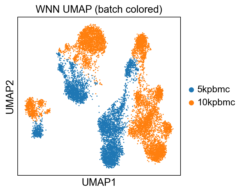
sc.pl.umap(rna, color='batch', title='WNN UMAP (batch colored)')

Which yields:

As well as running a leiden clustering on the weighted connectivities:

# clustering using WNN graph
rna.obsp['connectivities'] = rna.obsp['connectivities_wnn']
sc.tl.leiden(rna, key_added='leiden_wnn', resolution=0.5, neighbors_key='neighbors_wnn')
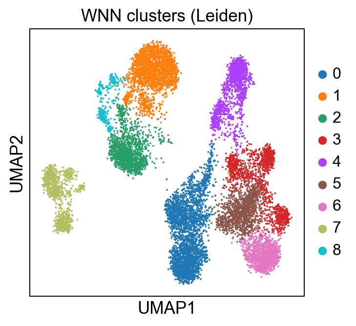
sc.pl.umap(rna, color='leiden_wnn', title='WNN clusters (Leiden)')

Giving us:

I am going to skip over the technical details a bit for brevity, but to help us evaluate the integration, let’s generate 3 more UMAPs:

1. RNA-only

2. Protein-only

3. WNN-integrated

These will allow us to visualize modality-specific structure, assess the success of the integration and serve as an entry-point for identifying any modality-specific artifacts:

# RNA-only UMAP
sc.pp.neighbors(rna, use_rep='X_pca', n_neighbors=N_NEIGHBORS)   # builds rna.obsp['connectivities']
sc.tl.umap(rna)
rna_umap = rna.obsm['X_umap']

# explicitly define dictionary for protein neighbors
prot.uns['neighbors'] = {
    'connectivities_key': 'connectivities_prot',
    'distances_key': 'distances_prot',
    'params': {
        'n_neighbors': N_NEIGHBORS,
        'method': 'umap'
    }
}

# protein-only: reattach connectivities to prot and umap
prot.obsp['connectivities'] = prot.obsp['connectivities_prot']
prot.obsp['distances'] = prot.obsp['distances_prot']
sc.tl.umap(prot, neighbors_key='neighbors')
prot_umap = prot.obsm['X_umap']

# WNN UMAP we stored as 'X_umap' on rna when computing with `neighbors_key='neighbors_wnn'`
wnn_umap = rna.obsm['X_umap']

# quick plotting
fig, axs = plt.subplots(1, 3, figsize=(12, 4))
axs[0].scatter(rna_umap[:,0], rna_umap[:,1], s=6, c=mdata.obs['batch']); axs[0].set_title('RNA-only')
axs[1].scatter(prot_umap[:,0], prot_umap[:,1], s=6, c=mdata.obs['batch']); axs[1].set_title('Protein-only')
axs[2].scatter(wnn_umap[:,0], wnn_umap[:,1], s=6, c=mdata.obs['batch']); axs[2].set_title('WNN integrated')
plt.tight_layout()

We get:

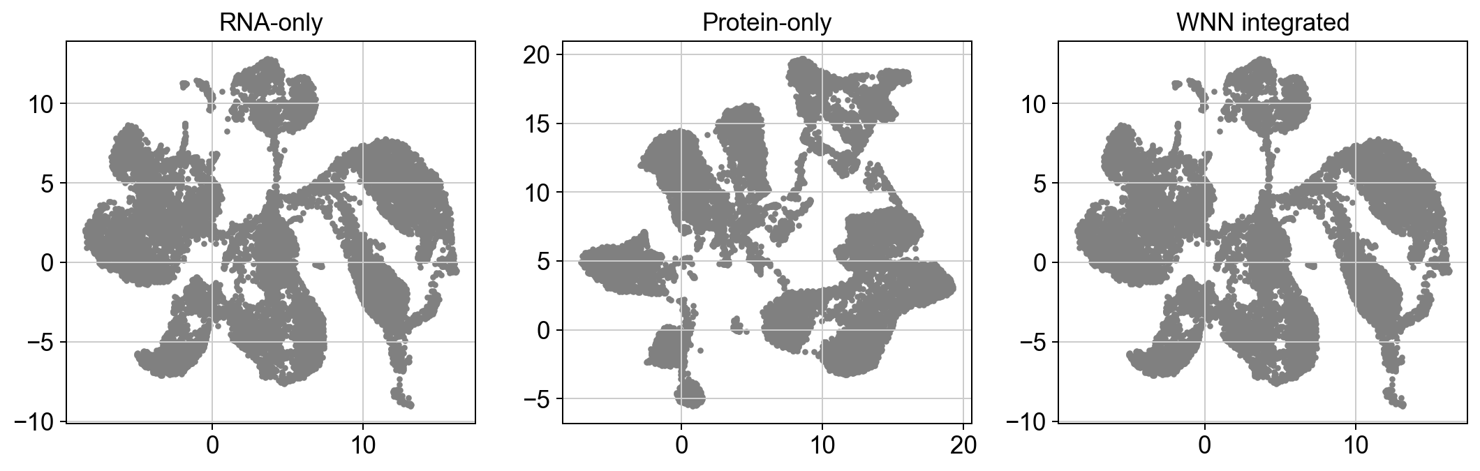
At an obvious glance, our WNN integrated plot looks eerily similar to our RNA plot. Because of this, we can say with somewhat certainty that the integration is dominated by RNA; which is less a question of that being good or bad, and moreso whether the data supports that hypothesis.

If our protein-only graph looked similar to the RNA graph, we could hypothesize that our protein features correlate strongly with our RNA features, so adding protein measurements didn’t add anything meaningful. But that isn’t the case.

So what do you think? Recall that our RNA and protein weights are slightly biased towards RNA. I challenge you to consider how adjusting the weights might shift these results. Additionally, explore the original dataset. Here’s another hint: we originally did an inner join on two datasets which wound up only sharing 17 proteins, compared to ~30,000 genes.

Our modality features are very obviously highly imbalanced. And our plots support that.

Which is a good thing!

Integration-only genes

Finally, let’s do a side-by-side marker gene comparison between clusters found using the RNA-only neighbors vs. the WNN-integrated neighbors, to see what extra biological information the integration adds. Step-by-step we’ll:

1. Cluster cells using RNA only

2. Find marker genes for RNA only

3. Find marker genes for WNN clusters

4. Pull the top marker genes

5. Compare the RNA-only vs WNN sets

# RNA-only clustering
sc.tl.leiden(rna, key_added='leiden_rna', resolution=0.5)  # using RNA-only neighbors

# rank genes in RNA-only and WNN clusters
sc.tl.rank_genes_groups(rna, groupby='leiden_rna', method='wilcoxon', key_added='rna_markers')
sc.tl.rank_genes_groups(rna, groupby='leiden_wnn', method='wilcoxon', key_added='wnn_rna_markers')

# get top N marker names for each cluster
def top_gene_set(adata, key, n=30):
    df = sc.get.rank_genes_groups_df(adata, group=None, key=key)
    top = df.groupby('group')['names'].apply(lambda s: list(s)[:n]).explode().tolist()
    return set(top)

rna_top = top_gene_set(rna, 'rna_markers', n=20)
wnn_top = top_gene_set(rna, 'wnn_rna_markers', n=20)
integration_only_genes = wnn_top - rna_top
print("Example integration-only genes:", list(integration_only_genes)[:20])

Now to plot the top 6 interaction-only genes:

# plot a gene that is integration-only
ex = list(integration_only_genes)[:6]
if ex:
    sc.pl.violin(rna, keys=ex, groupby='leiden_wnn', rotation=90, size=2)

And we get:

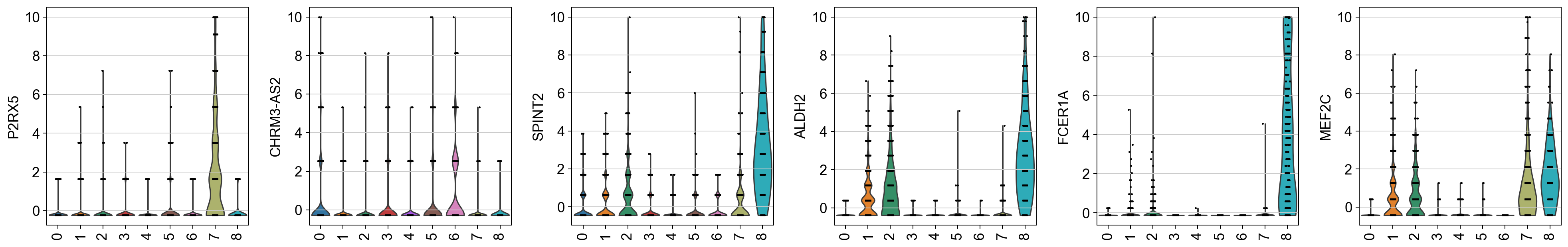
This serves as a check for whether integrating protein data into the neighbor graph changes which genes show up as top markers. Those additional markers might be subtle RNA features that only become important once we account for protein similarities in clustering.

Conclusion

We are in an era of atlas-scale multimodal data, acquired from millions of cells. Successful data integration has the potential to reveal biological function at a resolution yet unseen.

But multi-modal integration is hard.

It’s hard because biology is complex. It remains a challenge to capture modality-specific nuances (like scale, noise:signal ratio, pre-processing, batch effects etc.) and represent those in a single dimension i.e., in a single cell or sample. Not to mention, the most abundant protein may not correlate with high gene expression. This correlation (or lack thereof) makes integration difficult.

Be that as it may, this workflow is a gentle introduction to multimodal integration. Note that there are far more advanced (and perhaps more performant) methods out there like using TotalVI for joint probabilistic modeling, but those are less interpretable.

Though if you want to give those a shot based on this framework, go for it!

In our next lesson, we will take all we’ve learned about bioinformatics data types and multi-modal integration to scale, with an introduction to distributed computing and workflow engineering.

All code and supporting material here.